
The Swiss Labor Force Survey (SLFS) data is available to researchers by request, where each year’s data is provided as a large CSV file along with two additional sets of variable and value label files that have been exported from SAS and SPSS into TXT format. For those wishing to work with these label files in R, I introduce a few custom functions that transform the supplied label files into named objects that play nicely with the tidyverse haven and labelled packages.
Briefly on the SLFS
The Swiss Federal Statistics office (OFS) has conducted the Swiss Labor Force Survey (SLFS) since 1991 to gather representative data on the socio-economic structure of the country’s permanent resident population and their participation in the labor force. It’s based on a representative sample of the population, from which approximately 120,000 interviews are conducted annually. Prior to 2010 the phone based interviews (CATI) that make up the survey were all conducted in the second quarter of each year, but since that time, the interviews have been spread out to take place over the course of the entire year. The survey is fully compliant with international standards, covers the entire spectrum of standard labor market indicators, and includes a rotating set of thematic modules to investigate special topics of interest each year. For more details, just consult the French or German versions of the website, as the documentation is quite comprehensive.
Overview of the data
With regards to the survey data files themselves, prior to 2002, annual datasets typically include between 16,000 to 18,000 observations, but since that time, this number is more consistently in the 40,000 to 60,000 range. The organization and naming conventions used for the main CSV files are consistent over the years, with the one major change happening in 2010, where in addition to the annual data files, quarterly file subsets were included to reflect the change in the data collection process.
The variable names and values in the TXT label files show a bit more variation over time, so care should be taken to ensure that variable names and value label categories are consistent when putting together longitudinal panels using this data. Firstly, not all years have the same number of variables. For example, the files for the 1996 SLFS only capture a low of 507 different variables, while in 2006 there were up to 816 different variables measured (median across all years is 654).
Secondly, while most of the main variable names remain unchanged throughout the years, a few variable names are edited slightly to reflect updated methodologies or coding schemes. Just to name a few examples, the variable that records the commune of the respondent changes from B019 to B019P in 1999, or the variable that captures the different age groups off the respondents changes from AGE to AGE64 in 2001.
There are also cases where the variable names do not change at all, but the value labels used by the variables change as coding schemes are updated. One of the more notable examples is for the variable IS05 that records the national origin of the survey respondent. In 1996, the values of this variable changed from the old, 2-digit system where only 50 countries are captured, to the 4-digit system that captures the 200+ recognized country names currently used by the national statistical office today.
Importing the data with read_slfs
To work with the Swiss Labor Force Survey in R, I introduce three custom functions designed to read in the SLFS data (read_slfs), the variable label files (read_slfs_var) and the value label files (read_slfs_val) that are available on GitHub. All three depend on a number of other functions from the readr, stringr, tidyr, magrittr, tibble and the labelled packages. Those packages can be called up individually, or more conveniently, by just loading the tidyverse package along with the labelled package.
library(tidyverse)
library(labelled)
The read_slfs functions, themselves, can be downloaded directly from R by entering the following:
#install.packages(devtools)

devtools::source_url("https://raw.githubusercontent.com/anguyen1210/slfs-tools/main/R/read_slfs.R")
The main benefit of using these different read_slfs functions is to easily import the supplied SLFS variable and value label files into a format that is compatible with the different tools provided in the labelled package.
Working with single year files
The main data CSV file
The simplest case is reading in a single year of the SLFS data. As there is only a single data file, in CSV format, with a consistent naming convention for all years of the SLFS, this is straight-forward and can be done easily with the functions provided in base R or the readr package. Where the read_slfs function is different is that it can take up to 3 inputs: the SLFS data file, the variable label file and the value label file. If the respective label files are not included in the the read_slfs call, then the function just defaults to a simple readr::read_delim call.
In other words, the following two statements are equivalent when there are no other inputs:
read_slfs("data/SAKE1991.csv")

read_delim("data/SAKE1991.csv")
Before we see what happens when we try to read in everything at once, let’s first examine the two different label files that are included in these datasets.
The variable label files
The label files that are included with the SLFS data is where the bulk of the work needs to be done in order for everything to work in R. For each year of the SLFS, there are four sets of two label files provided–each set contains a variable label file and a value label file; with different sets for French and German labels, and different sets that are exported from SAS or from SPSS. These label files are available as simple TXT files, which is where the challenge lies.
While the haven package provides easy tools for reading in and working with SAS and SPSS files saved in their native formats (.sas7bdat and .sav files, respectively), the TXT exports of the respective label files have irregular formats that do not work with haven, nor with standard base R or readr functions.
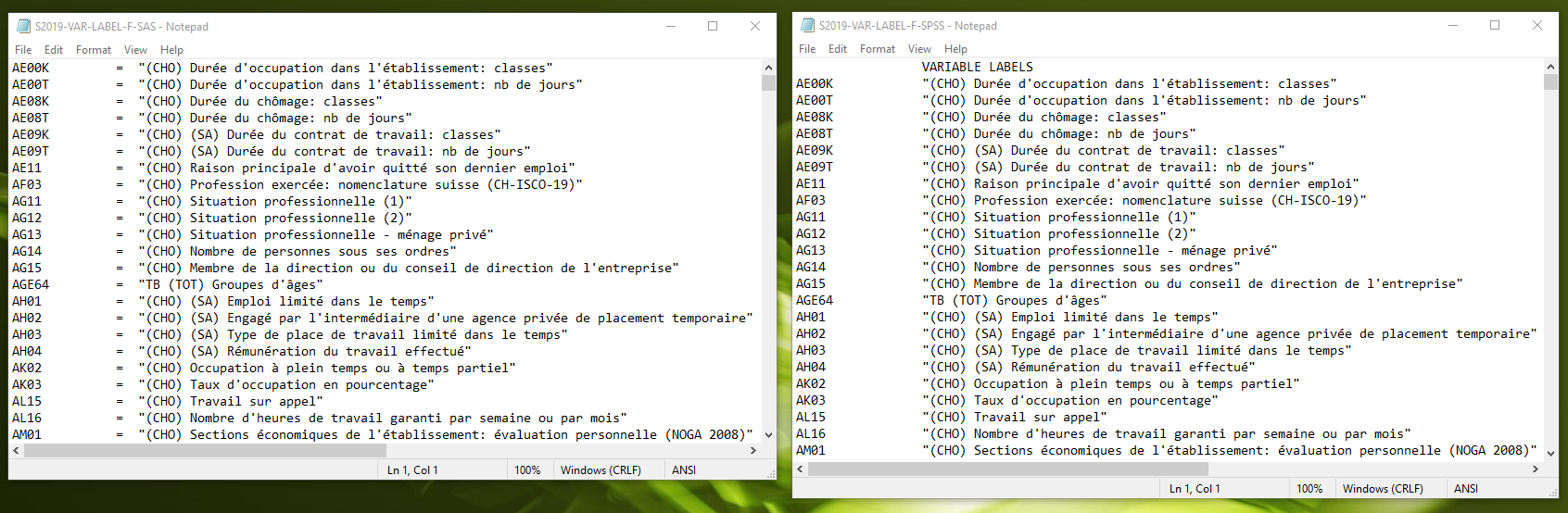
SAS- and SPSS-format variable label TXT files provided in the SLFS
Above we see the identical French variable label file in SAS format (on the left) vs. the SPSS version (on the right). The differences are minor–the SAS and SPSS version use different delimiters; the SPSS version has an extra offset line at the top and bottom of the file that must be accounted for.
read_slfs_var imports the respective label files and creates named character vectors that can then be fed into the different functions from the labelled package. read_slfs_var is indifferent to whether or not the SAS version or the SPSS version is provided as an input.
For example, the following imports of the variable label files for this year of the SLFS are equivalent:
varlab2019_sas <- read_slfs_var("data/S2019-VAR-LABEL-F.SAS.TXT")

varlab2019_spss <- read_slfs_var("data/S2019-VAR-LABEL-F.SPSS.TXT")
This is confirmed below, where we can see that the output using either input file is an identical named character vector:
glimpse(varlab2019_sas)## Named chr [1:692] "(CHO) Durée d'occupation dans l'établissement: classes" ...
## - attr(*, "names")= chr [1:692] "AE00K" "AE00T" "AE08K" "AE08T" ...glimpse(varlab2019_sas)## Named chr [1:692] "(CHO) Durée d'occupation dans l'établissement: classes" ...
## - attr(*, "names")= chr [1:692] "AE00K" "AE00T" "AE08K" "AE08T" ...sum(varlab2019_sas == varlab2019_spss)## [1] 692The value label files
With regards to the the SLFS value label files, while the SAS and SPSS versions are a bit more irregular then the corresponding variable label file, the read_slfs_val function also handles either one similarly and outputs an identical named list that can be used by the labelled package functions.
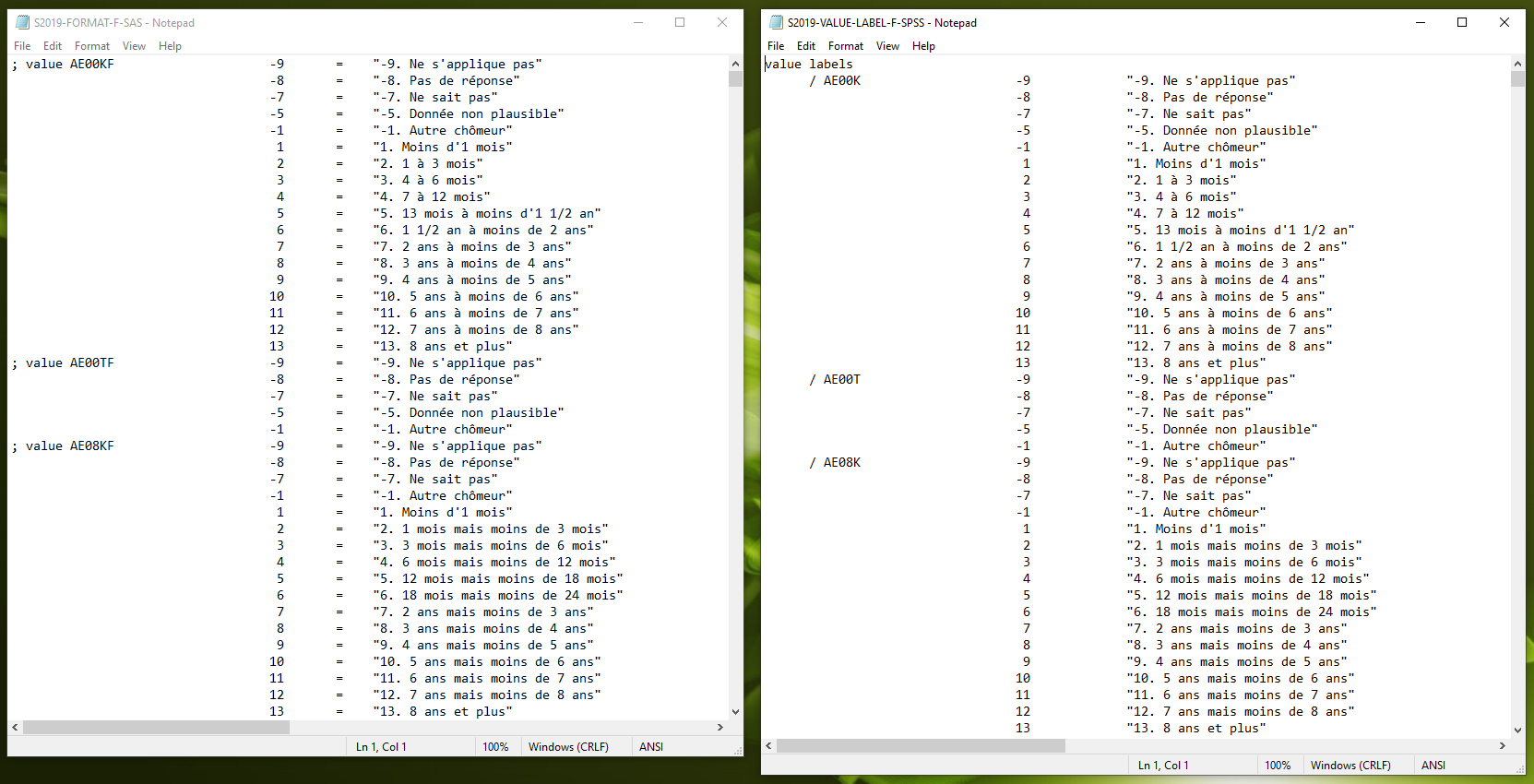
SAS- and SPSS-format value label TXT files
In this image above, we can see that there are a number of different little things that can trip up our import of these files, including the extra characters added to the SAS variables, the different delimiter scheme for the values in the SAS version, the added top and bottom line on the SPSS file. Regardless, we can read in either file the same was as before with read_slfs_val.
valuelab019_sas <- read_slfs_val("data/S2019-FORMAT-F-SAS.TXT")

valuelab019_spss <- read_slfs_val("data/S2019-VALUE-LABEL-F-SPSS.TXT")
As before, the output of read_slfs_val is identical regardless of whether the SAS or SPPS TXT file is used as an input. The difference here, however, is instead of a named character vector, the value label file is converted into a named list as we can see below.
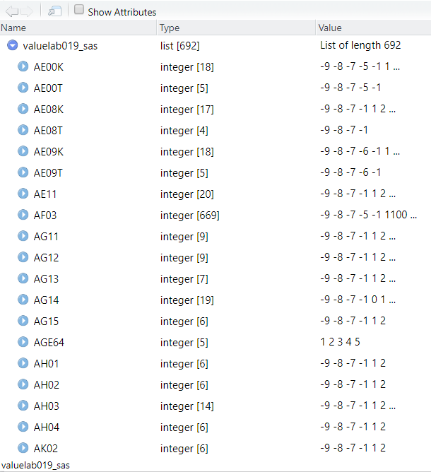
While it is possible to read in all of the label files in at the same time as the data file with the read_slfs function (as detailed below), I found it useful to have these label files imported as separate objects when I needed to quickly re-label subsetted data that had lost the initial labeling, or when I was in the process of doing a thorough analysis on the variables I had selected for analysis to see if and how they had changed over time.
Putting it all together
As I’ve already alluded to, it is possible to import the main data file and label all the variables and values at one time by supplying all three files (data, variable label and value label–in that order) to read_slfs at the same time.
slfs2019 <- read_slfs("data/SAKE1991.csv",
                      "data/S2019-VAR-LABEL-F.SAS.TXT",
                      "data/S2019-FORMAT-F-SAS.TXT"
                      )
slfs2019 %>% select(1:10) %>% glimpse()## Rows: 60,822
## Columns: 10
## $ AE00K <dbl+lbl> -9, -9, -9, -9, -9, -9, -9, -9, -9, -9, -9, -9, -9, -9, -...
## $ AE00T <dbl+lbl> -9, -9, -9, -9, -9, -9, -9, -9, -9, -9, -9, -9, -9, -9, -...
## $ AE08K <dbl+lbl> -9, -9, -9, -9, -9, -9, -9, -9, -9, -9, -9, -9, -9, -9, -...
## $ AE08T <dbl+lbl> -9, -9, -9, -9, -9, -9, -9, -9, -9, -9, -9, -9, -9, -9, -...
## $ AE09K <dbl+lbl> -9, -9, -9, -9, -9, -9, -9, -9, -9, -9, -9, -9, -9, -9, -...
## $ AE09T <dbl+lbl> -9, -9, -9, -9, -9, -9, -9, -9, -9, -9, -9, -9, -9, -9, -...
## $ AE11 <dbl+lbl> -9, -9, -9, -9, -9, -9, -9, -9, -9, -9, -9, -9, -9, -9, -...
## $ AF03 <dbl+lbl> -9, -9, -9, -9, -9, -9, -9, -9, -9, -9, -9, -9, -9, -9, -...
## $ AG11 <dbl+lbl> -9, -9, -9, -9, -9, -9, -9, -9, -9, -9, -9, -9, -9, -9, -...
## $ AG12 <dbl+lbl> -9, -9, -9, -9, -9, -9, -9, -9, -9, -9, -9, -9, -9, -9, -...Above, I show the first 10 columns of our imported data, where we can see that our data has fully labeled variables, as evidenced by the <dbl + lbl> class. Here, our data is ready to be used with the different helper functions provided in the labelled package.
Working with labeled files in R
The first thing that has to be said is that R does not handle labels in the same was as SAS, SPPS or Stata, so expectations should be tempered. When describing the use of labels and the “labelled” class, the authors of the haven point out that:
The goal of haven is not to provide a labelled vector that you can use everywhere in your analysis. The goal is to provide an intermediate datastructure that you can convert into a regular R data frame. You can do this by either converting to a factor or stripping the labels
With our main data file read in, along with its corresponding label files, the labelled package allows you to apply the labels to the data, sort the various labels and values, quickly reference label values, convert the labels to factors for use in plots, and any other number of operations.
For example, we can quickly check a variable label by entering the following:
var_label(slfs2019$B0000)## [1] "VA (ACT, APP, CHO, NA) Statut sur le marché du travail"Or supposing we see one of the observations in this column has a particular value, we can find the specific associated value label by entering:
val_label(slfs2019$B0000, 4)## [1] "4. Chômeur au sens du BIT"Or perhaps, we just want to quickly see the labels for all of the values of this variable, we can simply call:
val_labels(slfs2019$B0000)## 1. Actif occupé 2. Apprenti 4. Chômeur au sens du BIT
## 1 2 4
## 5. Non actif 6. Non-réponse
## 5 6As previously mentioned, there’s a lot you can do with the labelled package. Have a look at the “Introduction to labelled” vignette to get quickly up to speed.
Importing multiple years
In this final section, I demonstrate a quick solution to reading in multiple years of SLFS data and labeling everything at once, taking advantage of both read_slfs and purr.
Let’s say we want to load the last 10 years of SLFS data, and we uncompress all of the data we receive from the OFS so that the CSV files and their corresponding metadata subfolders all sit in the same folder (“/data”) as shown here:
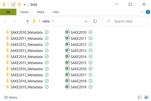
As we noted from before, the basic organization and naming conventions of the files are consistent over the years, and here we can see that the the file names are all identical apart from the year of the survey. With that said, we can quickly create a list for the different files that we want to read in, and then iterate over those lists to import all 10 years of the survey at once.
#specify the folder where your data is saved
fpath <- getwd()

# create lists of filenames
list_data <- list.files(fpath, pattern = "*.CSV", full.names=TRUE)

list_varlabs <- list.files(fpath, pattern = "*VAR-LABEL-F-SAS", full.names = TRUE, recursive = TRUE)

list_valuelabs <- list.files(fpath, pattern = "*FORMAT-F-SAS", full.names = TRUE, recursive = TRUE)
# read in data and label all variables and values at once, name the different
# data sets in the list
slfs2010_2019 <- pmap(list(list_data, list_varlabs, list_valuelabs), read_slfs)
data_names <- sapply(1:length(years), function(x) paste0("sake", years[x]))
names(slfs2010_2019) <- data_namesThe result is a list with all of the labeled datasets that we can easily work with, or collapse to one large dataframe with a simple bind_rows() call when ready.